Rows: 950
Columns: 1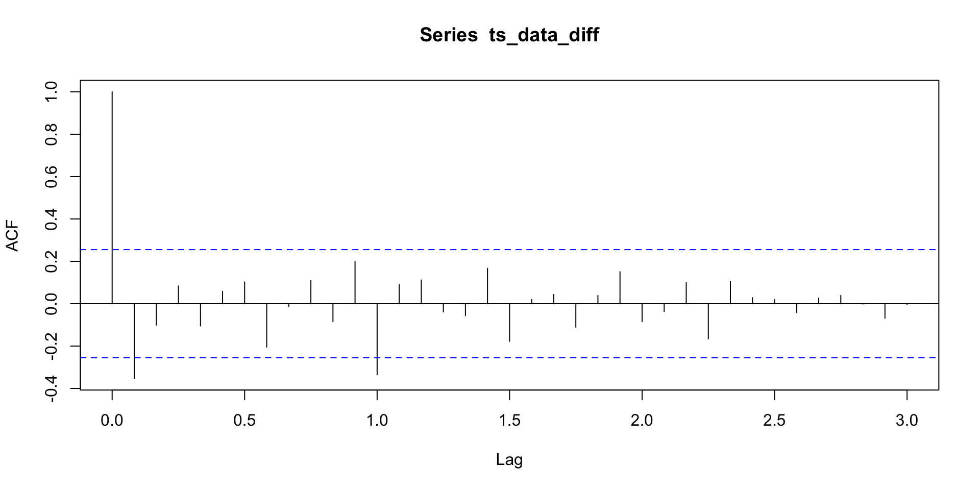
$ V1 <dbl> 4.587898, 4.165729, 2.003551, 1.347498, 3.484531, 3.766763, 4.62935…SARIMA
ME607 - Séries Temporais
SARIMA

SARIMA
\[\Phi(B^{12})y_t = \Theta(B^{12})U_t\]
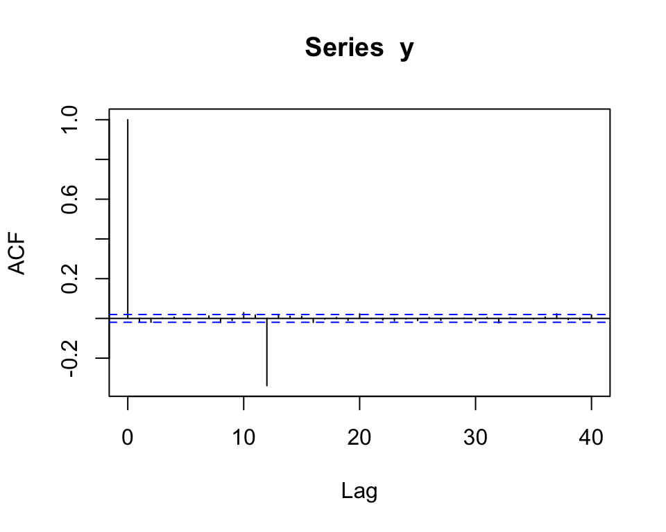
- Se \(Q = 1\), \(P = 0\) e \(\Theta_1 = -0.4\), então para as séries de cada mês em particular temos um \(MA(1)\).
- Se ademais \(\mathbb{E}(U_t U_{t+h}) = 0\), \(\forall h\) (ou seja, se as sequências para diferentes meses são não correlacionados entre si), então as colunas são não correlacionadas e a ACF seria da forma:
SARIMA
\[\Phi(B^{12})y_t = \Theta(B^{12})U_t\]
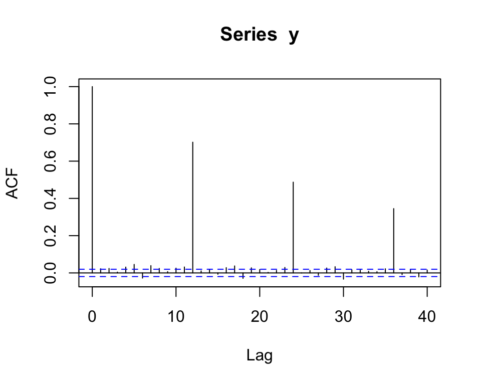
- Se \(Q = 0\), \(P = 1\) e \(\Phi_1 = 0.7\), então para as séries de cada mês em particular temos um \(AR(1)\).
- Se ademais \(\mathbb{E}(U_t U_{t+h}) = 0\), \(\forall h\) (ou seja, se as sequências para diferentes meses são não correlacionados entre si), então as colunas são não correlacionadas e a ACF seria da forma:
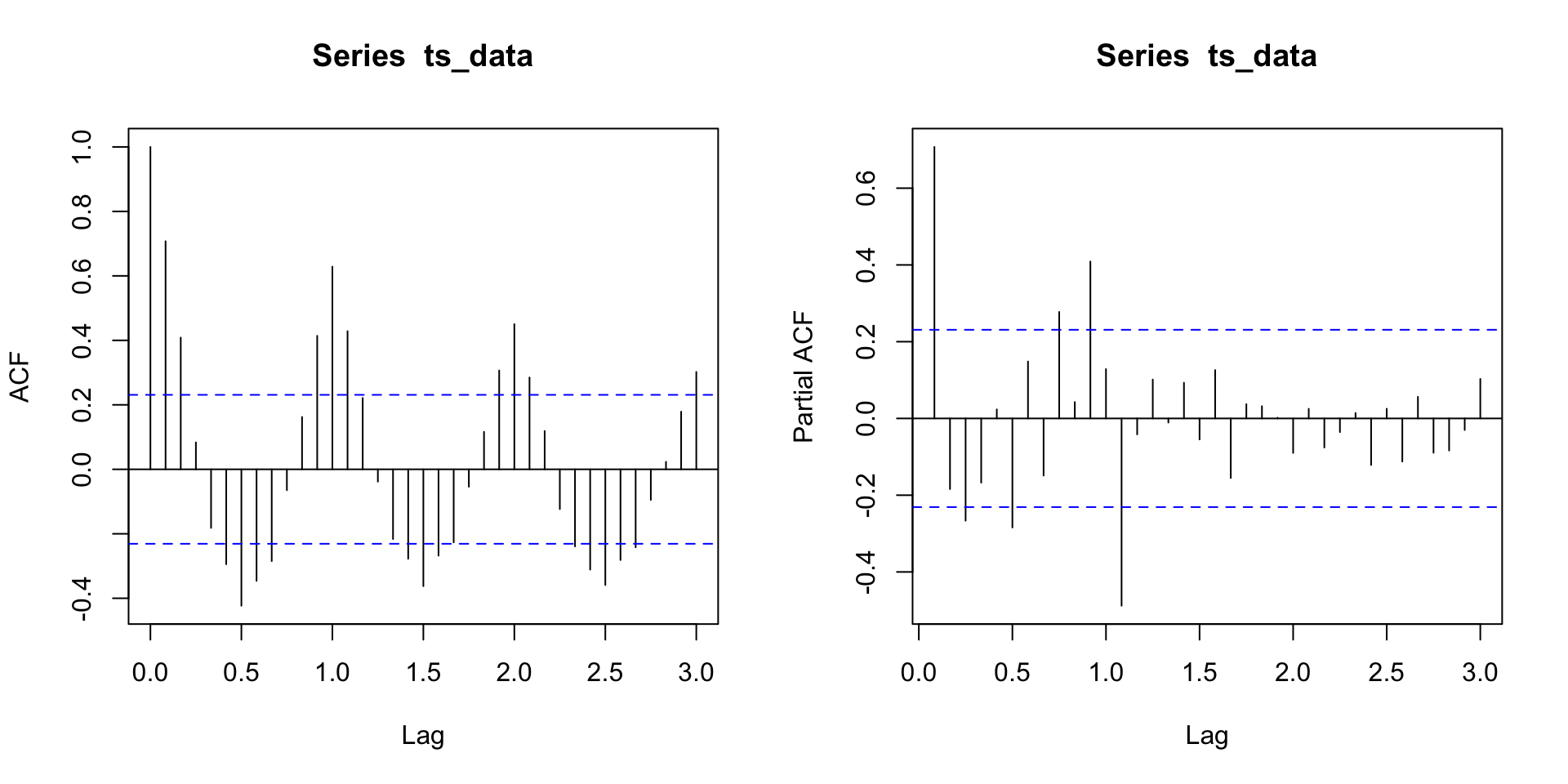
Mortes (mensais) acidentais US entre 1973 e 1978.
       Jan   Feb   Mar   Apr   May   Jun   Jul   Aug   Sep   Oct   Nov   Dec
1973  9007  8106  8928  9137 10017 10826 11317 10744  9713  9938  9161  8927
1974  7750  6981  8038  8422  8714  9512 10120  9823  8743  9129  8710  8680
1975  8162  7306  8124  7870  9387  9556 10093  9620  8285  8466  8160  8034
1976  7717  7461  7767  7925  8623  8945 10078  9179  8037  8488  7874  8647
1977  7792  6957  7726  8106  8890  9299 10625  9302  8314  8850  8265  8796
1978  7836  6892  7791  8192  9115  9434 10484  9827  9110  9070  8633  9240
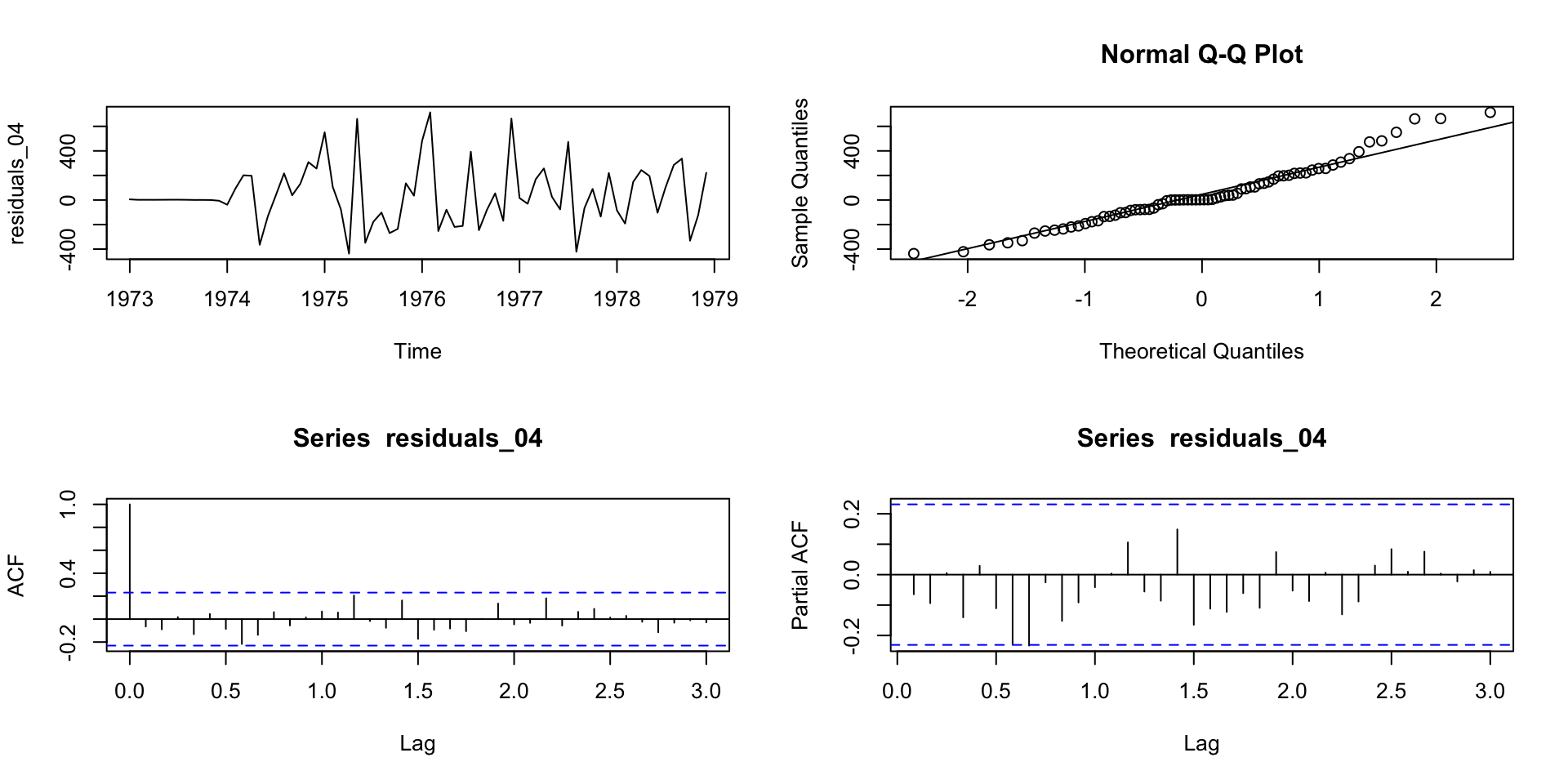
SARIMA \((0, 1, 1) \times (0, 1, 1)_{12}\)
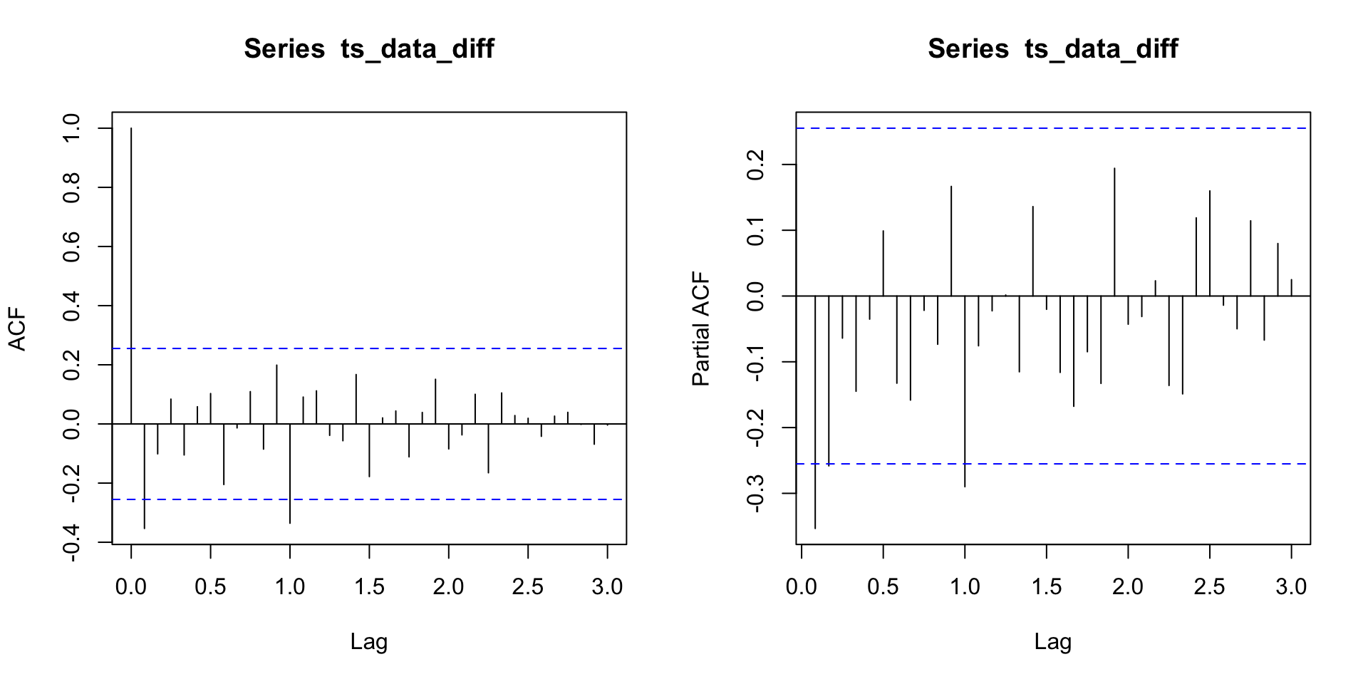
Mortes (mensais) acidentais US entre 1973 e 1978.
- E se eu não tiver certeza que \(p = 0\), \(q = 1\), \(P = 1\) e \(Q = 1\)?
- Um SARIMA \((0, 1, 1) \times (0, 1, 1)_{12}\) é um \(MA(q + sQ) = MA(13)\) com restrição, né? Então, porque não ajustar um \(MA(13)\)?
- Observação: como temos poucos dados, utilizaremos apenas métricas dentro da amostra. Se tivéssemos muitos dados, poderiamos fazer um rolling window e ver qual faz melhor previsão.
Code
 [1] 873.7457 868.4179 864.6874 866.6413 868.4728 863.6197 860.2355 862.2132
[9] 864.3034 859.6358 857.2329 859.3756 865.4692 860.9361 858.6464 860.8906[1] 11 p q P Q
1 0 0 0 0
2 1 0 0 0
3 0 1 0 0
4 1 1 0 0
5 0 0 1 0
6 1 0 1 0
7 0 1 1 0
8 1 1 1 0
9 0 0 0 1
10 1 0 0 1
11 0 1 0 1
12 1 1 0 1
13 0 0 1 1
14 1 0 1 1
15 0 1 1 1
16 1 1 1 1
Call:
arima(x = ts_data, order = c(0, 1, 13), seasonal = c(0, 1, 0))

Coefficients:
          ma1     ma2      ma3      ma4     ma5      ma6      ma7      ma8
      -0.4166  0.0947  -0.0592  -0.0707  0.2439  -0.2881  -0.0624  -0.0233
s.e.   0.1582  0.2072   0.2264   0.2523  0.2284   0.2367   0.1660   0.2157
         ma9    ma10    ma11     ma12    ma13
      0.0514  0.1455  0.0458  -0.6686  0.3867
s.e.  0.2193  0.2428  0.2182   0.2289  0.2123

sigma^2 estimated as 79206:  log likelihood = -421.76,  aic = 871.52
. . .
Code
Call:
arima(x = ts_data, order = c(0, 1, 13), seasonal = c(0, 1, 0), fixed = c(NA,
0, 0, 0, NA, NA, 0, 0, 0, 0, 0, NA, NA))
Coefficients:
ma1 ma2 ma3 ma4 ma5 ma6 ma7 ma8 ma9 ma10 ma11
-0.5018 0 0 0 0.2604 -0.2209 0 0 0 0 0
s.e. 0.2074 0 0 0 0.1703 0.1890 0 0 0 0 0
ma12 ma13
-0.9289 0.2032
s.e. 0.2492 0.1830
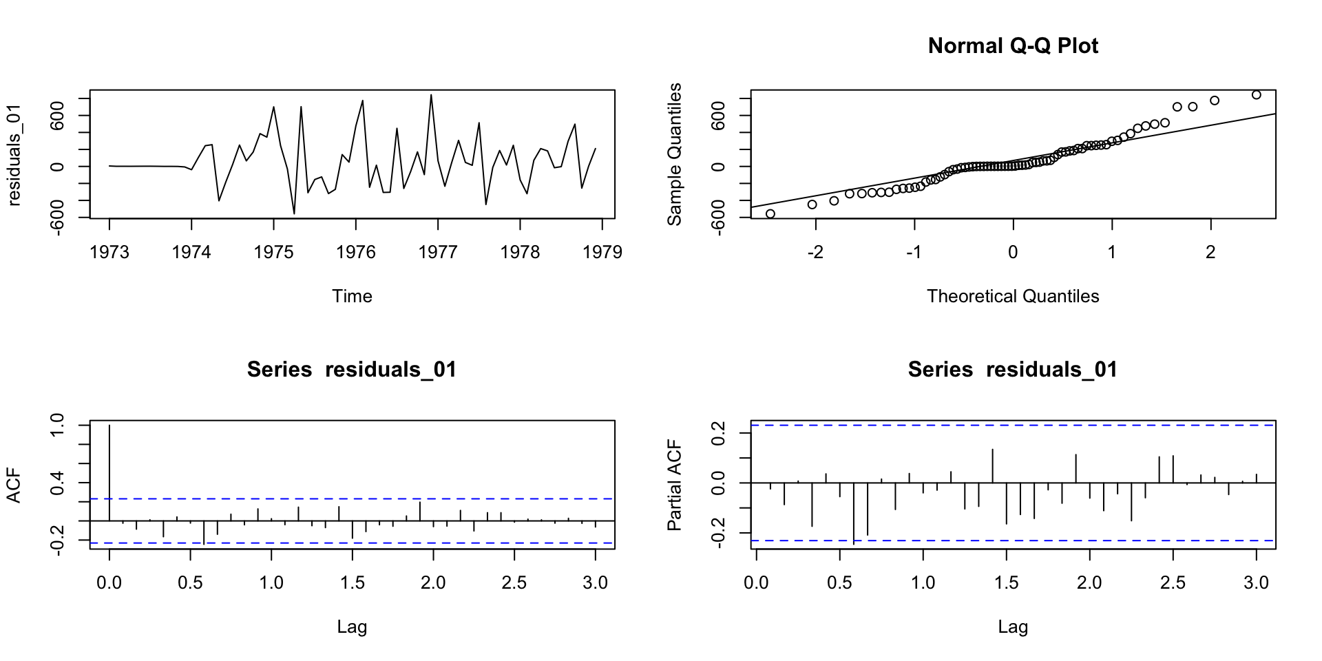
sigma^2 estimated as 66822: log likelihood = -422.64, aic = 857.27Code
Call:
arima(x = ts_data, order = c(0, 1, 13), seasonal = c(0, 1, 0), fixed = c(NA,
    0, 0, 0, 0, 0, 0, 0, 0, 0, 0, NA, NA))

Coefficients:
          ma1  ma2  ma3  ma4  ma5  ma6  ma7  ma8  ma9  ma10  ma11     ma12
      -0.5180    0    0    0    0    0    0    0    0     0     0  -0.8833
s.e.   0.2235    0    0    0    0    0    0    0    0     0     0   0.3295
        ma13
      0.1323
s.e.  0.2018

sigma^2 estimated as 75607:  log likelihood = -424.92,  aic = 857.83
[1] 857.2329 878.8892 864.6387 865.2017